Pearson correlation coefficient, coefficient of determination

Pearson correlation coefficient For a population

For a sample

coefficient of determination (\(R^2\))

Definition: the proportion of the variance in the dependent variable that is predictable from the independent variable(s).

When we test the models performance, \(R^2\) measures the size of the residuals from the model compared to the size of the residuals from a null model (mean value). On the training data, as the model cannot be worse than the null model, \(R^2\) will always be positive. It may not be the case for the testing data as the model can do worse than the null model.

some notes

Things above are some basics that we all know. However, recently colleagues of mine proposes that our traditional approach of evaluating our prediction model’s performance is problematic.

Previously, when we want to evaluate our model, we will first use cross-validation to generate predicted values and then calculate its Pearson correlation (\(r\)) between predicted vs observed values. However, when we do this, \(r\) reports the degree to which the predictions are correlated with observations, this is not the same as \(R^2\) where it represents the accuracy of the model.

In the training set, when we regress observations (\(\bar{y}\)) on the predicted values (\(\hat{y}\)), the model will simply be \(y=\hat{y}\) as the regression model already assures to minimize residual sum of squares (SSR) and \(\hat{y}\) is already the linear combination of predictors. So there is no additional fitting when we evaluate the model on training data. \(r\) will just be the square root of \(R^2\).

However, in the testing data, when we calculate \(r\), we are actually fitting a secondary model \(y=a+b\hat{y}\), and this will result in a higher \(R^2\) than we can get from directly apply the definition equation of \(R^2\). Some test set observations have gone to the secondary model which inflates the result. So reporting this secondary \(R^2\) may not give you what you think you want.

All of this is tricky and if we want to say that \(R^2\) is the explained variance of the model, we have to make sure that “the model” is the one we trained, not the nontrivial secondary model.

在买这辆civic si之前其实我已经开了一年的civic hatchback，但是因为一次他人的过错，那辆hatchback报废在了我家门口，本着“本田大法好”的信仰，我毫不犹豫地又购入了这辆更加心仪的si，目前来看，我并不后悔这个决定。

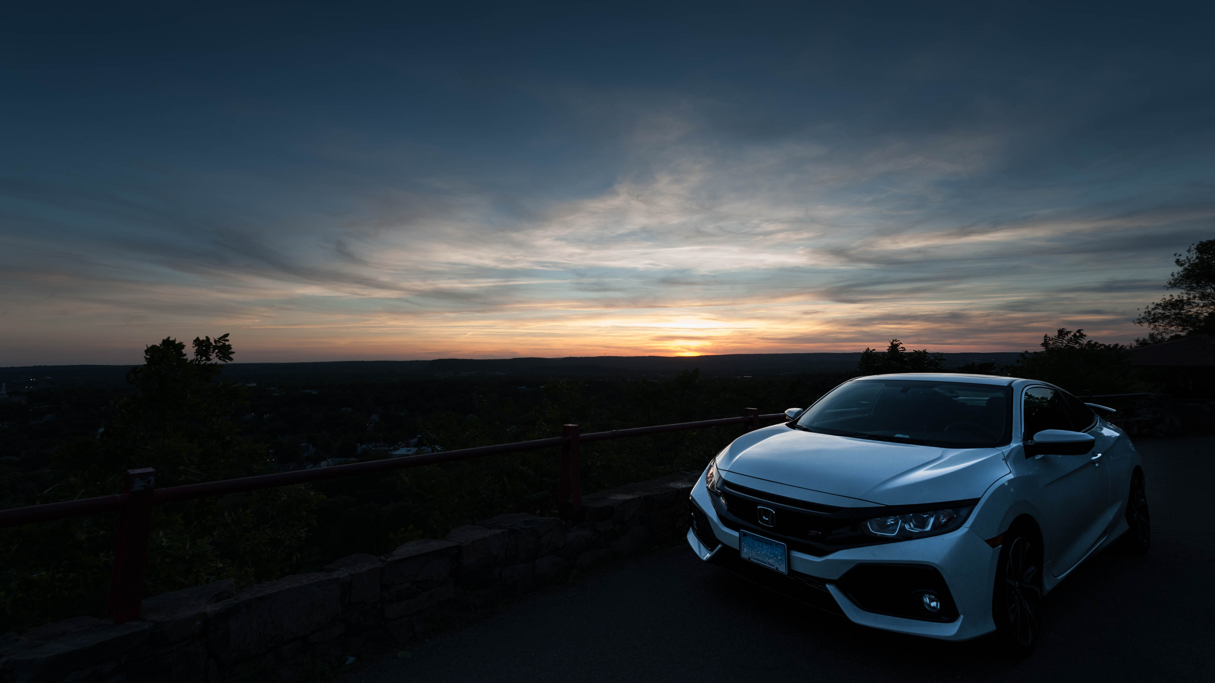@ East rock park, sunset

外观内饰

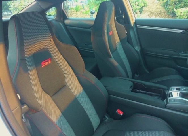
在买第一辆车之前，我算是一个80%的外观党，尽管一直有关注各种汽车方面的咨询，但是毕竟买车前也只有500km的驾驶经验，要我真的因为某些看起来虚无缥缈的“驾驶体验”来买车还是很难的，所以我能判断的也就是像外观内饰这样的比较简单就可以确定个人偏好的东西。而这辆si，我对他的外观可以给9分了，如果考虑到价格，那绝对是同级别里我心中的9.9分，10分留给gti。 但是内饰，不好意思，只能给到6分，而且这6分有很大程度是因为这个包裹性不错而且印有红色si logo的座椅。其他部分，infotainment system, 嵌有carplay，所以在娱乐方面还是不错，但是自带的honda系统真的丑+难用。反人类的音量调节触摸滑条再一次印证了“不要轻易在低端车上使用先进硬件”的真理。而且把空调调节功能也集合在娱乐系统的屏幕上让我成功的放弃了自己调节车内空调的习惯，因为系统打开时候的卡顿，auto模式成为了我常年的选择。一直很好奇为什么这些大的汽车厂商不能认真优化一下自己的UI，现在手机厂商满地起，为什么不能也顺便入侵一下这些传统行业呢？可能carplay是最终一个很好的解决方案，但是作为汽车厂商，也不应该放任其他厂商控制自己车内重要的驾驶交互环节。 最后吐槽一下各方面的做工，不论是方向盘按钮，还是后备箱或者手套箱，都有着一种浓浓的廉价感，而且这种体验是在摸过了同样日系的q50后逐渐加深的，于是现在每次用方向盘上的控制按钮的时候，都有一种“好好赚钱买好车”的冲动。

操控

说到操控，先要表扬下这次si只给了手动挡的配置，所以买车的时候没有什么犹豫的，直接手动挡走起。

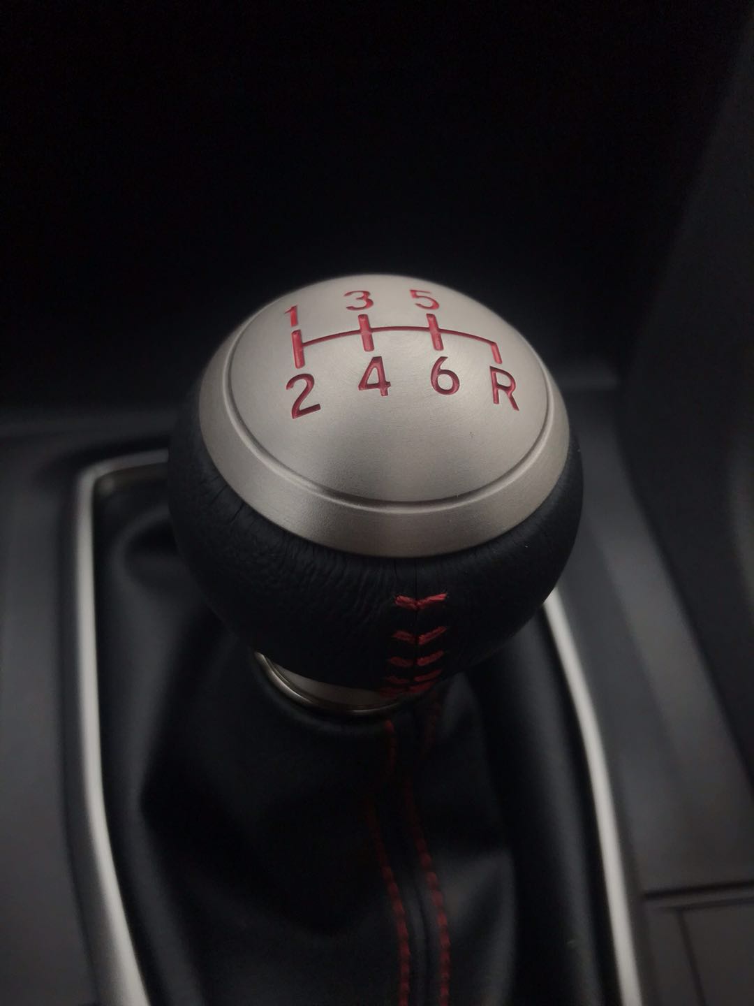
非常喜欢这款si的换挡杆，乒乓球型金属挡杆手感非常润滑，换挡手感清晰干脆，而且每次换挡结束有种独特的吸入感，真的让人欲罢不能，记得刚买完这辆车的时候，经常会熄火以后再玩上几分钟的换挡杆。。

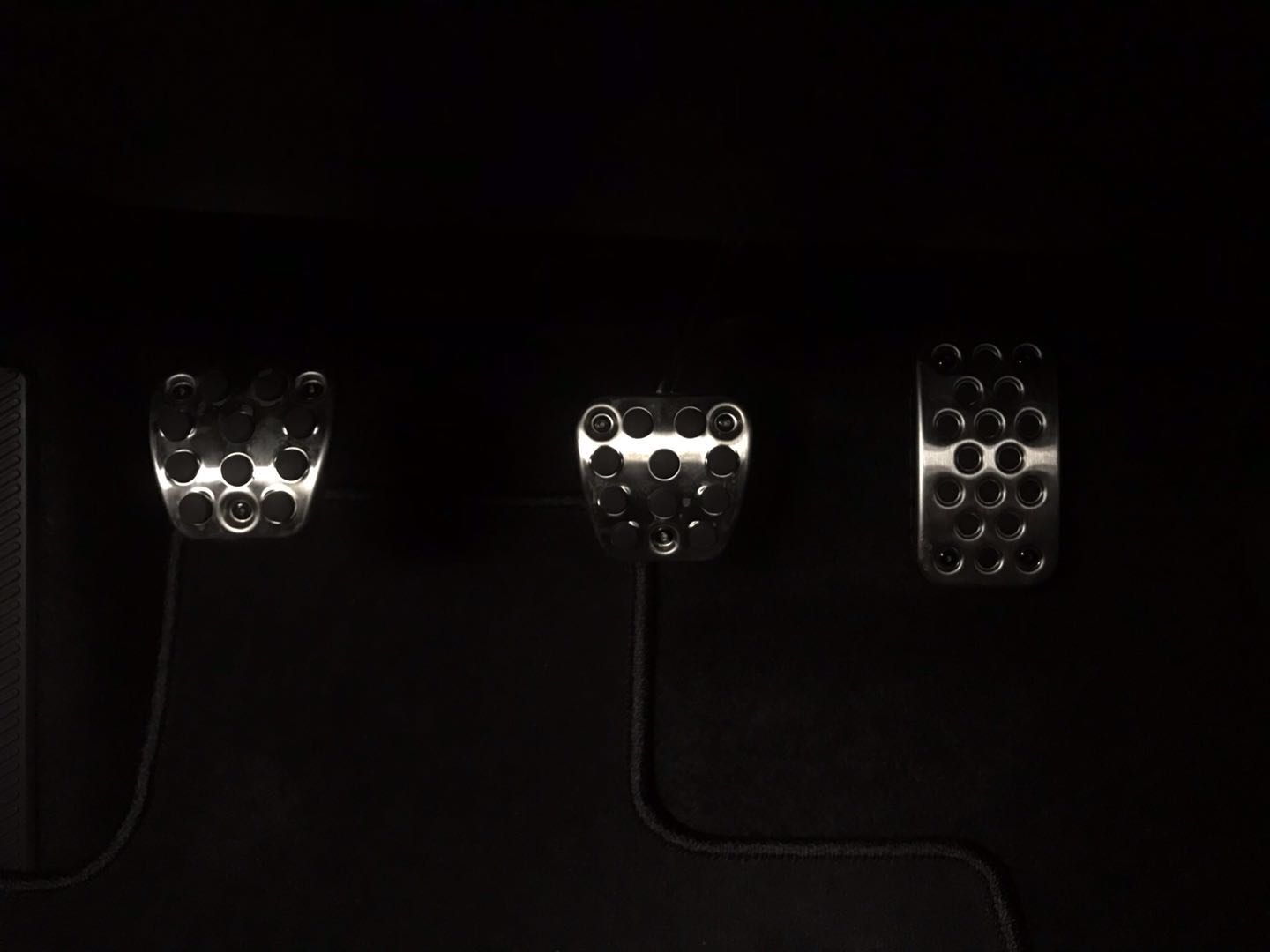
比起换挡杆的出色手感，踏板位置就有点尴尬了，因为油门和刹车踏板距离太远，导致跟趾基本没办法做。看视频好像可以后脚跟放在油门踏板后面，然后脚掌斜挎油门刹车踏板从而在后脚跟稳定的情况下做跟趾，这个还需要练习。离合的感觉相对来说就要好很多，非常的轻而且结合点非常好找，在刚开始练习熄火几次之后基本就不再有问题了。

动力上来说，因为手动挡的关系，让我对加速有了更多的欲望和控制，所以这也就让这辆si可以在城市或者高速路上路口轻松加到我需要的速度，而且每一次换挡前强烈的吸力配合上换挡后略微把身体向前推的惯性，让人欲罢不能。当然必须要吐槽的一点是这辆车的rev hang比较令人烦恼，尤其是1挡换2挡想要平顺的话必须要等一会松离合，好像这个功能与燃油经济性有关还是什么，通过ktuner好像可以解决这个问题，等我攒够钱可以尝试一下，如果消除了rev hang，那起步速度应该会有很大的提升。

其实把这辆si和普通的civic拉开差距的地方对我来说就是前轮的限滑差速器（LSD）了，虽然我还没有激烈测试过LSD和open-differential的区别，但是可以感觉出来配备了LSD的si在让我过发卡弯这种道路时有了更强的信心而且从来没有出现过打滑的问题。

其他

空间真的有点小，用这个车搬了两次家，苦不堪言，但是后备箱的空间还算decent，不过总体来说之前的hatchback要实用的多。

油耗在这个定位的车来说真的挺良心的，对于我这种经常暴力驾驶并且对于空调和音乐音量有着变态追求的人来说，27+mpg的油耗真的算不错了。

电子手刹有点失去了拉手刹独有的快感。

1. Lin’s Kitchen
2. Lao Sze Chuan
3. Formosa Asian fusion
4. lobster hut (lobster rolls)
5. Takumi Japanese cuisine.
6. mocha noodle bar (chicken wings)

@ New York

1. Pocha32 (love the Korean ramen there)
2. His and her (Chinese dessert)

@ Buckhead, Atlanta

1. Southern City Kitchen Buckhead (fried chicken is awesome)
2. True Food Kitchen (tataki is awesome)
3. Poor Calvin’s (lobster fried rice there is tasteful with Asian enough flavor)
4. Seven lamps (lobster buns is fresh… omg I love lobster)

@Phoenix, Arizona

1. Dust Cutter (avocado fries there is good, also the chicken and waffle)

@ 杭州 Hangzhou（排名分先后）

1. 你别走（小龙虾）
2. 臻货（海鲜）
3. 台海岸（椒盐虾）
4. 火狐狸（川菜）
5. 塔哈尔（新疆菜）
6. 菲滋 （芝士条）
7. 夏星酒馆（排骨年糕火锅）
8. 淮扬菜馆扬州龙虾（麻辣小龙虾）
9. 大鸡腿
10. 普罗旺斯（法餐）

Learning slow is due to the shape of the sigmoid function.

When we use sigmoid function, then the partial derivative of the quadratic cost function for the weight and bias are multiplied by \(\sigma'(z)\). For example, when the desired output is near 0 while the actual output is 1, then the learning is slow although the neuron’s performance is bad.

[] As we can see, the curve tends to be flat when Z is bigger.

Thus, we need a better function than the trivial quadratic cost function. And cross-entropy is one of the alternatives. The cost function is \(C = -\frac{1}{n} \sum_x \left[y \ln a + (1-y ) \ln (1-a) \right],\) With some algebra calculation, we can prove that the partial derivative of the cost function for weights and bias is independent of \(\sigma'(z)\). And it is only related with \(\frac{\partial C}{\partial w_j} = \frac{1}{n} \sum_x x_j(\sigma(z)-y),\)

And it is worth noting that

the cross-entropy is nearly always the better choice, provided the output neurons are sigmoid neurons.

Basis function

By inserting knots, we got more piecewise cubic polynomials to fit, which enables us to fit more complex functions.

However, without constraint on the border, we may undergo discontinuity on the boundary. To fix this problem, we can (1) force the polynomial to be continuous at the knot by modifying our model (2) we can add indicator functions or truncating function $(x_i-c)_+$ to make a uniform equation.

By this will only make the knot point continuous but not no continuous derivative. So we add the continuity condition on the first&second derivative of the function.

We can also add additional constraint to two ends of the curve.

We should also pay attention to the position of knots and how many knots should we put. Cross-validation can be used to choose the number of knots.

Week10

• Nearest neighbor doesn’t suffer from over-fitting as regression that much.
• Gini index can be used to measure the importance of variable in tree-based classifiers.
• gbm package for boosting
• Default variable numbers tried in “randomforest” package tried:

  if (!is.null(y) && !is.factor(y))
    max(floor(ncol(x)/3), 1) 
  else 
    floor(sqrt(ncol(x)))
  

• Bootstrapping generates multiple trees and bagging summarizes them together.
• Randomforest uses different subsets of variables at each iteration.
• Boosting tree added variables sequentially.
• One easily-made mistake for randomForest package is that, when the levels of train and test data are not the same, like if you have a variable with level==[0,1] but it all equals 0 in the test set, then there will be a problem when you predict the test set using the trained model. So you have to preset all the predictor levels in the test set equal to the ones in training set.